Once all the information has been captured, as we saw in the first part of this post, 3D scanning with drones (I): data capture, we move on to processing that data
Processing the information
There are several software packages for data processing: some are cloud-based, others hybrid, and so on. I will just mention a few of them, since choosing one or another depends on several factors and is not the purpose of this section. In the end they are all fairly similar in terms of the results we are after and how they process the data. Their biggest difference is the pricing model: some have a perpetual licence, some a monthly or annual subscription and others charge per project or by credits. Depending on how many projects with these needs we take part in, one package or another will suit us better.

Notable among them are Autodesk's Recap, DroneDeploy's own cloud-based software and the one we will use here in its desktop version, Agisoft Methasape.
With that said, let us start on our case study, which alternates images from two examples: the foundation stage of a detached house and a ruined building.
Loading the images
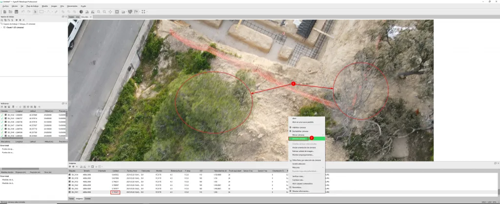
First, we add the drone photos to our software. Once they are loaded, the software lets us review their quality using a set of internal algorithms that assign a value between 0 and 1. Any photo with blurred areas, heavy overexposure or motion blur will score below 0.7, and 0.8 is the minimum we should accept if we want our generated model to be free of inaccuracies.
Aligning the photos
Workflow>Align Photos.
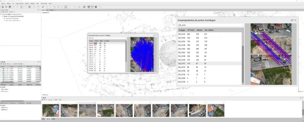
This generates a sparse point cloud. Essentially, it finds matching points between photos so that they can be paired (this is where the overlap we set up in our flight mission becomes important). Once the sparse point cloud has been generated, we can review those matching points.
The image below shows how, compared with the same photo (DJI_0151), 3524 matches were found, of which 2802 were valid and 452 invalid. For the same photo, on the other hand, only 110 points were found, of which 67 were valid and 43 invalid. Data like this, where valid points are very low compared with invalid ones, help us judge whether we need to take more shots on site with the drone or whether we can carry on with the processing.
Once this is done, and before processing our dense point cloud, the software lets us resize the working volume, in case we are not interested in part of the terrain and want to save processing time.
Building the dense point cloud
Workflow>Build Dense Cloud
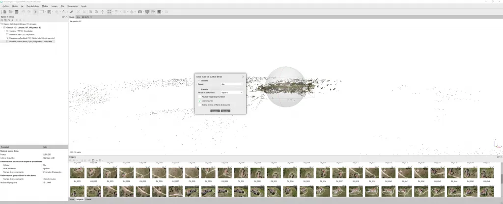
When generating our dense point cloud, the options under Depth filtering are worth highlighting. They determine how information that is insignificant because of its size in the model will be filtered out. For example, if we are processing a church with a small cross on its bell tower, mild filtering will keep it, whereas aggressive filtering will remove it.
Ground control points
No ground control points were used in these examples, as we did not need a particular level of accuracy in our models and were not going to georeference them. Even so, it is one of the most critical steps, since the accuracy of the exported model depends on it.
To georeference and scale the model, when flying the drone we need to place several markers on the ground that can then be easily identified in the software. These points are surveyed with topographic equipment to obtain their coordinates, which we then use to adjust the points in our photographs. Between 5 and 7 control points will be enough for situations like this one.
Explaining how to bring these control points together in Metashape would take a whole post of its own, so we will stick to the theory of why we need them.
Classifying the point cloud
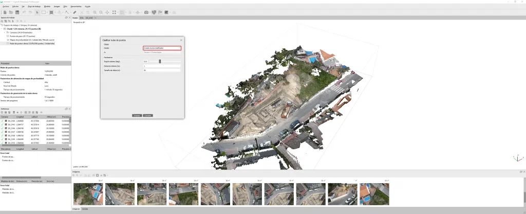
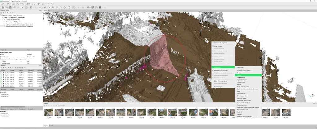
Tools>Dense Cloud>Classify Ground Points.
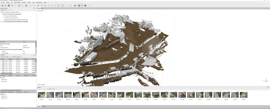
Here we classify every element that is ground and separate it from everything that is not. Once the ground has been marked, we can filter out everything that is “not ground”, such as buildings, machinery, trees and so on, and assign it a category.
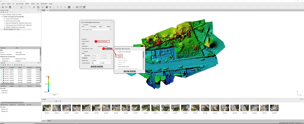
With this distinction in place we can generate digital terrain models instead of digital elevation models. The latter would distort our measurements, since we would get contour lines that include the tree canopies, for example.
Building the overall surface model
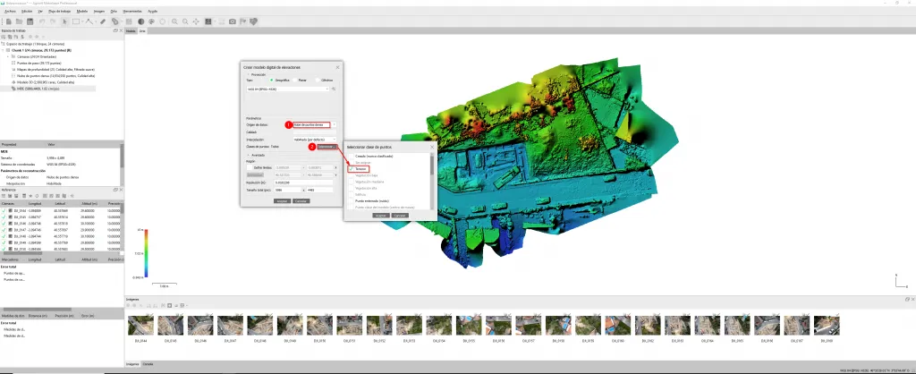
Workflow>Build DEM
If we have filtered our dense point cloud as explained in the previous step, our ground will be separated from existing buildings, vegetation, vehicles and so on. This helps us generate an overall elevation model filtered to show only what we are interested in (in our example, just the ground).
Generating the orthomosaic and exporting contour lines
Workflow>Build Orthomosaic
This is the step we need to take first if we want to export the terrain contour lines to AutoCAD, for example.
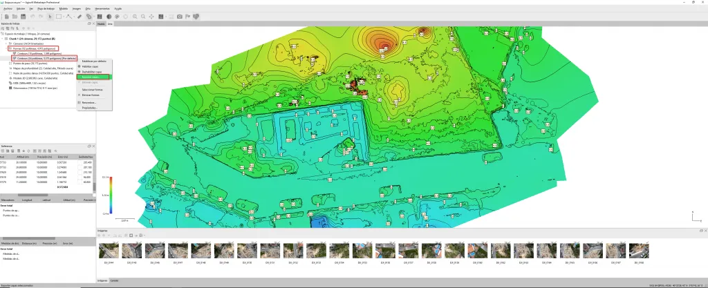
Under Tools>Generate Contours… we add the contour lines to our model, choosing the minimum and maximum elevation to generate and the interval between them.
In our workspace (left-hand panel), Shapes drop-down>Contours (the contour lines we have generated)>Export Layers… we choose .dxf as the output format and the file is created in the chosen location.
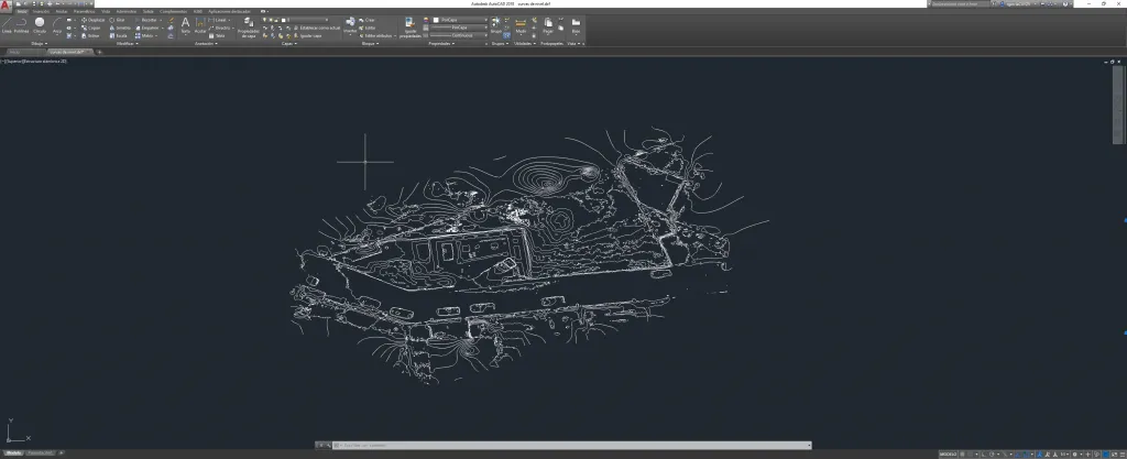
The model could be clipped to a specific area if we did not want to export the whole extent of the contour lines. In our case we kept things simple and generated the raw information, which looks like this, ready to be imported into other software such as Revit.
Finally, if we want to import our point cloud into Revit, we need an intermediate step through Recap (there are other options, but this is the simplest).
In the workspace panel, right-click the dense point cloud>Export Dense Cloud… A window opens with various export options. We choose the one that suits us best, open Recap and import it. We make any corrections needed, such as adjusting coordinates, and save.
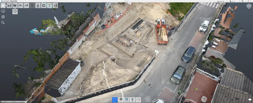
Once we have our file in .rcp format, all that remains is to import the .rcp point cloud into Revit.
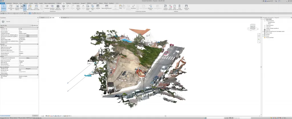
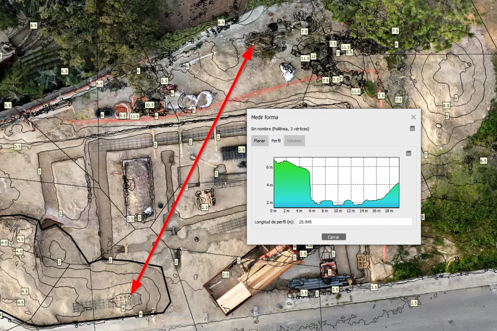
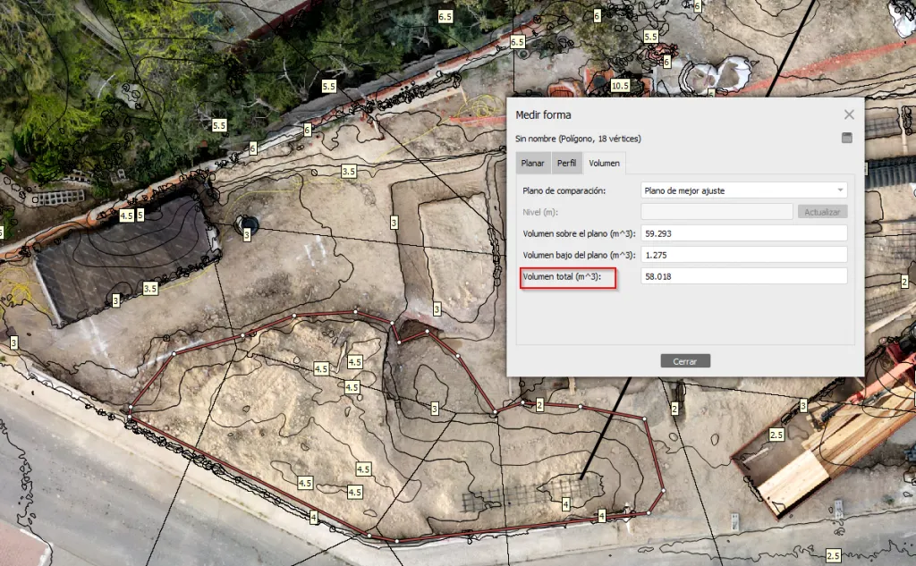
And that completes the whole workflow. Needless to say, this has only been a small example: the potential of this software lets us do more complex things, such as merging aerial surveys with ground surveys carried out with other types of scanner (Faro/Leica), or taking simple measurements on the model, such as the change in level along a section through the terrain or the volume of a drawn polygon.